
arrange.m(arrange objectsinside a figure) |
 p = arrange(n) returns a length n cell array of 4 element vectors
specifying the positions of n objects covering most of the current figure. This is useful for positioning the screen objects
during the initial design phase of a graphical interface. Although this produces a haphazard layout, you can then
use the mouse to size and position the objects, which is easier than numerically specifying explicit locations for each object.
Two examples that show how to do this appear in the
p = arrange(n) returns a length n cell array of 4 element vectors
specifying the positions of n objects covering most of the current figure. This is useful for positioning the screen objects
during the initial design phase of a graphical interface. Although this produces a haphazard layout, you can then
use the mouse to size and position the objects, which is easier than numerically specifying explicit locations for each object.
Two examples that show how to do this appear in the
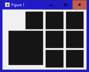
Suppose we test the arrange function by typing the following line into the command prompt:
plt('box',arrange(8));
This will produce the figure shown to the right. Notice
that the first box is placed in the lower left corner and is four times the area of the other boxes. It's intended that you
use p{1} (the first location generated) for the application's main plot (if there is one). Of course,
you will likely move and resize this anyway, but it is easier if the main plot starts bigger than its supporting elements.
b64decode.m(base64 decoder) |
Decodes the file named infile that was encoded using base64 encoding and saves it in a file named outfile. Most programs with a similar function contain at least one loop, but b64decode, true to good Matlab style, does not use any loops. (Of course we should use loops when they simplify the code, but this is a good example where loops offer no advantage.)
outfile may also contain just the extension of the output file.
For example:
b64decode('c:\path1\abc.txt','.exe') creates the output file c:\path1\abc.exe
If the second argument is not provided, '.bin' is assumed.
See erip.m as an example of the use of this function to automatically convert the supplied base64 encoded text file iir.b64 to create the iir.zip archive (which contains the iir.exe executable).
datestr(serial datenumber to ascii) |
a = now;
| datestr(a,13) | 03:51:46
| plt('datestr',a,13) | 03:51:46.153
| datestr(a,14) | 03:51:46 AM
| plt('datestr',a,14) | 03:51:46.153 AM
| datestr(a,0) | 31-Mar-2015 03:51:46
| plt('datestr',a,0) | 31-Mar-2015 03:51:46.153
| datestr(a) | 31-Mar-2015 03:51:46
| plt('datestr',a) | 31-Mar-15 03:51:46.153
| |
dealv.m(deal vector) |
[e1 e2 e3] = dealv([77 66 55]); is equivalent to the three lines:
e1 = 77;
e2 = 66;
e3 = 55;
This is similar to Matlab's deal function, except for vectors instead of cell arrays. For examples of the use of this function, see the programs demo\wfall and sig\editz.
figpos.m(figure positioning) |
Consider the following two methods of creating a new figure window:
figure('BackgroundColor',[0 0 .1],'Position',p);
figure('BackgroundColor',[0 0 .1],'Position',figpos(p);
In the first method, the pixel coordinates in p are relative to the full screen which especially with a multi-window GUI makes it impossible to make good use of the screen area without knowing where the taskbar is and other desktop variables. In the second line however, the coordinates in p are relative to a pre-defined clear area of the screen which are converted into absolute screen coordinates by figpos (this routine).
To accomplish this, figpos must know the screen area that can accommodate the Matlab figure window. It gets this information from the screencfg.m routine which normally can determine this information automatically. (See the description of the screencfg function below.) screencfg saves this information in a text file as well as in an application data variable so that it doesn't have to recalculate the screen configuration the next time it is called. If you move or resize the taskbar figpos will continue to return positions consistent with the old taskbar position. To fix that problem, after moving the taskbar, type figpos('reset') or the command form figpos reset in the command window. This causes figpos to recalculate the screen configuration to take account of the new taskbar size and location.
First, I will explain how figpos computes the figure position from the input argument, although you may find it easier to understand by skipping ahead to the examples below.
In rare situations, you may want to specify the screen position using the standard Matlab convention [left bottom width height] referenced to the screen without reference to the border areas. Of course, then you don't need to call figpos in the first place ... except for the fact that figpos is called automatically by plt, so we need a way to bypass the usual figpos processing. The way to do that is simply to place an "i" after any element in the 1x4 vector. For example:
figpos([40 50i 600 500]) returns the vector [40 50 600 500].
It doesn't matter which element contains the "i", and in fact you can put the "i" in all 4 elements if you like, i.e. figpos([400 50 600 500]*1i);
Suppose you call figpos([p1 p2 p3 p4]) where all the terms are real and p3 and p4 are both positive. This is called "size priority mode" because getting the figure size correct takes priority over getting the left/bottom position in the specified place. In this mode, figpos will return [left bottom width height] where:
   width  = the smaller of p3 and the maximum clear width available
   height = the smaller of p4 and the maximum clear height available
   left   = p1 + left border width. However, if this position would make the
            right edge of the figure overflow the clear space available, then
            the left edge is moved rightward just far enough so the figure fits.
   bottom = p2 + bottom border width. However, if this position would make the
            top edge of the figure overflow the clear space available, then
            the bottom edge is moved down just far enough so the figure fits.
Suppose you call figpos([p1 p2 -p3 p4]), i.e. the same as the calling
sequence above except that the 3rd element is negative. The height and
bottom values are computed exactly as shown above (size priority), but
the width and left values are now computed as follows (position priority):
   left   = p1 + left border width.
   width  = p3. However, if this width would make the right edge of the figure
            overflow the clear space available, then the width is reduced by
            just enough so that the figure fits.
Suppose you call figpos([p1 p2 p3 -p4]), i.e. the 4th element is negative.
The left and width values are computed exactly as shown in the first all
positive (size priority mode) but the bottom and height values are now
computed as follows (position priority):
   bottom = p2 + bottom border width.
   height = p4. However if this height would make the top edge of the figure
            overflow the clear space available, then the height is reduced
            by just enough so that the figure fits.
If you call figpos([p1 p2 -p3 -p4]), then both horizontal and vertical
coordinates use the position priority method described above.
An optional 5th value in the input vector is allowed to allocate extra space for the title bar. You may want to do this if you know that a menu bar or toolbar will be enabled since that will make the title bar larger. Since this is not accounted for in the screen configuration set up by screencfg, enabling these features could cause the top edge of the figure to fall off the top edge of the screen. For example:
figpos([p1 p2 p3 p4 48]) would allocate 48 extra pixels in the vertical space which would be enough for the menu bar (about 21 pixels high) and one toolbar (about 27 pixels high).
The default left/bottom coordinates are [5 5] which are used if they are not supplied. For example:
figpos([700 500]) gives the same results as figpos([5 5 700 500]).
figpos([700 500 48]) gives the same results as figpos([5 5 700 500 48]).
You also may specify only the figure length or the figure width and let figpos calculate the missing size parameter based on the most appropriate aspect ratio. For example figpos([1000 0]) and figpos([0 944]) both give the same results as figpos([1000 944]). This particular aspect ratio (1.006) was chosen so that if you plot a circle, the resulting figure is actually looks circular rather than elliptical. For example, this line plots a perfect circle using 600 points:
plt(exp((1:600)*pi*2i/599),'pos',[800 0])
The following examples may clarify the specification described above:
The first example creates 5 plots of the same size placed on the screen so that all the plots are as far away from each other as possible. The first four plots are placed right at the edge of the screen at the four corners, except not so close that any of the figure borders disappear and of course not obscuring the taskbar no matter where the taskbar is placed. On a small screen, even the first four figures would overlap. On a large screen, the first four figures would not overlap, but the fifth figure would overlap the corners of the other four (unless the screen had an exceptionally high resolution).
   y = rand(1,100);  sz = [700 480];     % data to plot and figure size
   plt(y,'pos',[ 0   0  sz]);            % bottom left corner
   plt(y,'pos',[Inf  0  sz]);            % top left corner
   plt(y,'pos',[ 0  Inf sz]);            % bottom right corner
   plt(y,'pos',[Inf Inf sz]);            % top right corner
   p = get(findobj('name','plt'),'pos'); % get positions of all 4 plt figures
   plt(y,'pos',mean(cell2mat(p))*1i);    % put 5th plot at the average position
The "*1i" in the above line is necessary to prevent figpos from
adjusting the position using the current border information. The raw pixel
location is used because the get('pos') command returns raw pixel coordinates.
With the "*1i" removed, the last figure would not be at the exact arithmetic
mean position (although possibly the error might be too small to notice.
The next example also creates four figures at the corners of the screen, although this time, the first figure is a fixed size, and the remaining figures are tiled to fill all the remaining space on the screen.
   plt(y,'pos',[ 0   0   600  400]); % figure 1 is placed at the lower left corner
   plt(y,'pos',[ 0  440  600 -Inf]); % use all the remaining space above fig1
   plt(y,'pos',[615  0  -Inf  400]); % use all the remaining space to the right of fig1
   plt(y,'pos',[615 440 -Inf -Inf]); % use all the remaining space not used by figs 1-3
Note that in the example above an extra 15 pixels in width and 40 pixels in height is used to create a small gap between the four figures.
figpos may also be called with one of the following string arguments:
| figpos('reset') | Because the screen configuration is saved, you must execute this command after moving the taskbar. Otherwise, figures will not be positioned based on the old taskbar position. |
| figpos('full') | Returns the position coordinates of the largest figure possible that doesn't overlap the taskbar.
To create such a figure use the command:
|
| figpos('width') | Returns the width of the figure mentioned above |
| figpos('height') | Returns the height of the figure mentioned above |
In addition to the examples above, a good way to appreciate the value of the figpos function is to run demoplt.m and cycle thru all the plt demo programs using the "All Programs" button. Notice how well the various windows are placed on the screen. You will appreciate the intelligence of the placement even more, if you can rerun the demos using a different screen resolution and a different taskbar location. Without the figpos function, many of the demos would have to be more complicated to place their figures at appropriate screen positions.
funcStart.m(spawn afunction) |
carlo run
circles12
curves go
fseries go
movbar run
pltmap run
wfall run
(Note, the optional argument 'run' or 'go' tells the application to start updating the moving image as soon as it starts.) Using a straightforward implementation of such a GUI program, the program would run continuously to update the moving image and therefore the command prompt would not reappear in the command window after starting the program. This means that you couldn't enter any more Matlab commands in the command window until the GUI program terminated, or the program was instructed to stop updating the figure. The funcStart function provides a way to initiate the moving image and return immediately so that the command window is again able to accept new Matlab commands. The eight programs listed above serve as examples of how to use funcStart to achieve this objective.
funcstart(@func,d);
funcstart({@func arg1 arg2 ...},d);
If funcStart is nested less than d levels below the command prompt then funcStart calls function @func (with arguments if supplied) and then returns to the calling function immediately without waiting for @func to complete. If funcStart is called from a more deeply nested function, then @func is called but it doesn't return to the calling function until @func is complete.
funcstart(@func);
funcstart({@func arg1 arg2 ...});
When called without the 2nd argument, d defaults to 2. This means that after @func is initiated, execution of the calling function will continue immediately only if funcStart was called from the command prompt or from the top level of a script or function. Otherwise @func is called but it doesn't return until @func is complete.
Because @func is called as a timer function callback, two extra arguments are added at the beginning of the argument list. This means that arg1 will actually be the 3rd argument of @func and arg2 will be the 4th, etc.
Note: If you don't care about the nesting depth you can use funcstart(v,Inf);
matplt.m(.mat fileplotting) |
Refer to that section as a guide to how to use the resulting figure.
Examples:
| matplt('c:\mcode\plt\ini\myfile.mat') | Opens the specified file with full path information |
| matplt('c:\mcode\plt\ini\myfile') | Same as above |
| matplt | Presents a dialog box so you can choose a file |
| matplt('myfile.mat') | Searches the path for the specified file and opens it if it's found. If it's not found, matplt behaves as if it was called with no arguments. |
| matplt('myfile') | Same as above |
| matplt myfile | Same as above (command form) |
metricp(metricprefixes) |
When called with two arguments, this is used to convert a number to a form using standard metric prefixes. pfix is the metric prefix string that is most appropriate for displaying the value x, and mult is the x multiplier. This is often useful for scaling plots to avoid awkward scientific notation in the axis labels.
x = .3456E-6;
| sprintf('%.3e Volts',x) | 3.456e-007 Volts
| [pfix mult] = plt('metricp',x);
| sprintf('%.1f %sVolts',x/mult,pfix) | 345.6 Nano-Volts
| |
The metric prefixes used and their respective multipliers are as follows:
| Kilo | 103 | Milli | 10-3 | Exa | 1018 | Atto | 10-18 |
| Mega | 106 | Micro | 10-6 | Zetta | 1021 | Zepto | 10-21 |
| Giga | 109 | Nano | 10-9 | Yotta | 1024 | Yocto | 10-24 |
| Tera | 1012 | Pico | 10-12 | Ronna | 1027 | Ronto | 10-27 |
| Peta | 1015 | Femto | 10-15 | Quetta | 1030 | Quecto | 10-30 |
When called with more than two arguments, this is used to change or query the metric prefixes used for the x or y axis of a plot:
| xm = plt('metricp',ax,'x'); | Update Xaxis metric prefix. Returns new x multiplier |
| ym = plt('metricp',ax,'y'); | Update Yaxis metric prefix. Returns new y multiplier |
| [xm ym] = plt('metricp',ax,'both'); | Update both X and Y axis metric prefixes |
| [xm ym] = plt('metricp',ax,'get'); | Get current axis multipliers |
| plt('metricp',ax,'-x'); | Reset Xaxis multiplier to 1 |
| plt('metricp',ax,'-y'); | Reset Yaxis multiplier to 1 |
| plt('metricp',ax,'-both'); | Reset both X and Y axis multipliers to 1 |
The first three commands re-adjust the metric prefixes based on the current axis limits. So for example, if the current axis limits are [0 4300], the limits will be changed to [0 4.3] and the metric prefix will be bumped to the next level (from Kilo to Mega for example) and the line data will be divided by 1000.
For an example of how to use the metricp function to update the metric prefixes to accommodate changes in the plotted data, look at the carlo.m application in the math folder.
Pftoa.m(float to ascii) |
If fmtstr is of the form '%nW' then swill be the string representation of x with the maximum resolution possible while using at most n characters.
If fmtstr is of the form '%nV' then
swill be the string representation of x with the
maximum resolution possible while using exactly n characters.
If fmtstr is of the form '%nw' then
s will be the string representation of x with the
maximum resolution possible while using at most n characters -
not counting the decimal point if one is needed.
If fmtstr is of the form '%nv' then
s will be the string representation of x with the
maximum resolution possible while using exactly n characters -
not counting the decimal point if one is needed.
The lowercase formats (v,w) are typically used to generate strings to fit into gui
objects of a fixed width. The reason the decimal point is not counted is
that with the proportional fonts generally used in these gui objects, the
extra space taken up by the decimal point is insignificant.
With all four format types, if the field width is too small to allow even one significant digit, then
'*' is returned.
fmtstr may also use any of the numeric formats allowed with sprintf.
For example:
Pftoa('%7.2f',x) is equivalent to sprintf('%7.2f',x)
Normally Pftoa must include exactly two arguments, but there is one exception.
The command Pftoa('test') or equivalently Pftoa test will
create a test file called PftoaTest.txt. Looking at the examples in this text file may help
you better understand the differences between the four new format specifiers.
Normally you won't call Pftoa directly since calling it thru
prin is more general and just as concise.
(See prin below.)
prin.m(sprintf& fprintf alternative) |
s = prin(FID,fmtstr,OptionalArguments);
Converts the OptionalArguments to a string s using the format specified by fmtstr. Note that this does the same thing as sprintf or fprintf (with the same calling sequences) except that prin offers some additional features including four extra formatting codes. prin calls the Pftoa function described below to implement the new formatting codes. FID is usually a value returned from fopen but can also be a 1 or a 2 to direct the result to the Matlab command window. For a complete description of this function, see prin.pdf (in the plt\util folder). You can view that help file most quickly by simply typing prin (i.e. with no arguments) at the Matlab command prompt.
pp.m(pretty printerfor vectors & matrices) |
pp(matrix);
The array pretty print capability is actually built into prin but pp gives you quick access to this useful capability. Type pp or prin without any arguments to see the full documentation (pdf file). The pretty printing feature is described in the last two pages of the document.
pltpub.m(publication plots) |
| The 'COLORdef',0 parameter | to select a white plot background |
| The 'TraceID','' parameter | to remove the TraceID box |
| The 'NoCursor' option | to remove the cursor objects |
| The '-All' option | to remove the menu box |
The demo programs pub0.m, pub1.m, and pub2.m, and xChart.m demonstrate the use of pltpub and also shows that any of the pltpub defaults may be overridden.
If the first pltpub argument is 'Cpick' (as done in the pub0 and xChart demos) then the ColorPick action is assigned to all plt lines, axes, and text elements. This makes it easy to make final color adjustments before the screen capture. It also has the (usually desirable) side effect that all mouse-driven zoom and pan operations are disabled. (Don't include this argument if you need those mouse-driven operations.)
Consider creating your own functions similar to pltpub with sets of plt defaults that you use frequently.
pltt.m(add plt trace) |
Pvbar.m(verticalbar plots) |
plt(Pvbar([2 3 7 8],0,[6 6 5 1]);
Normally all three Pvbar arguments are vectors of the same length, however in this case since the lower y position
of each bar is the same a constant may be used for the 2nd argument.
Although you don't have to know this to use it, Pvbar returns a complex
array that is interpreted correctly by plt or plot to display the desired
sequence of vertical bars. plt and plot displays complex arrays by plotting
the real part of the array along the x-axis and the imaginary part of the
array along the y-axis. The trick that Pvbar uses to display a series of
lines with a single array stems from the fact that NaN values (not a number)
are not plotted and can be used like a "pen up" command. (The Pebar
and Pquiv functions described below use this same trick.)
The general form of the Pvbar function call is:
v = Pvbar(x,y1,y2)
If the inputs are row or column vectors, this would return a complex
column vector which when plotted with plt or plot would produce a series of vertical
bars (of the same color) at x-axis locations given by x. y1 and y2 specify the lower and
upper limits of the vertical bar. It doesn't matter whether you list the upper or lower
limit first. If y1 is a scalar, Pvbar expands it to a constant vector of the
same size as y2.
Suppose you wanted to plot 30 red bars (specified by length 30 column vectors xr,yr1,yr2)
and 30 green bars (specified by length 30 column vectors xg,yg1,yg2).
You could do this with two calls to Pvbar as in:
plt(Pvbar(xr,yr1,yr2),Pvbar(xg,yg1,yg2));
That's probably the first way you would think of, but if xr and xg happen
to be the same length (as in this case) you can accomplish the same thing
with a single call to Pvbar:
plt(Pvbar([xr xg],[yr1 yg1],[yr2 yg2]));
The second form is especially convenient when plotting many bar series
(generally each series in a different color). Interestingly, if you use plot
instead of plt first form will not work so you must use the second form.
Note that Pvbar will expand the second argument in either dimension if
needed. So for instance in the example above, if ya1 and yb1 were the same
you could just use ya1 as the second argument. Or suppose the base (lower
limit) of the first series was always 0 and the base of the second series
was always -1. Then you could use [0 -1] as the second argument. If the base
of all the bars in all the series was the same value, then the second
argument may be a scalar.
To see Pvbar in action, look at the
Pebar.m(error barplots) |
The general form of the Pebar function call is:
e = Pebar(x,y,l,u,dx)
The position of the bottom of the error bars is y-l and the top is y+u. The last argument (dx) is a scalar that specifies the width of the horizontal Ts as a percentage of the average x spacing. The last two arguments are optional. If dx is not specified it defaults to 30 (%). If u is not specified it defaults to l (the 3rd argument) in which case the reference coordinates become the midpoints of the error bars. e,x,y,l,u are generally vectors or matrices of the same size, the only exception being that l and u are are allowed to be scalar. Read the description of Pvbar above for an explanation of how vector and matrix inputs are interpreted.
To see Pebar in action, look at the
Pquiv.m(vector plots) |
plt(Pquiv([4;2;1],[9;3;7],[0;0;1],[1;-1;0]));
This can also be done using Pquiv's complex input form as follows:
tail = [4+9i;2+3i;1+7i]; head = [1i;-1i;1];
plt(Pquiv(tail,head));
Note that row vectors could have been used instead of column vectors if desired. Now suppose in addition to those 3 vectors, you wanted to plot 3 more vectors (in a second color) with the same tail locations but pointing in the opposite direction. Using the previous assignments of tail and head, This could be done as follows:
plt(Pquiv(tail,head),Pquiv(tail,-head));
Or you could do the same thing with a single call to Pquiv:
plt(Pquiv(tail*[1 1],head*[1 -1]));
Of course, the equivalent 4 argument (real input) form of Pquiv could have been used as well.
There are 8 possible calling sequences for Pquiv depending on whether the input arguments are real or complex and on whether the optional arrow head size argument is included. Pquiv is smart enough to figure out which calling sequence you are using.
| Calling sequence | Tail coordinates | Arrow width/length | Arrow head size |
| q = Pquiv(A,B) | [real(A), imag(A)] | [real(B), imag(B)] | 0.3 |
| q = Pquiv(A,B,h) | [real(A), imag(A)] | [real(B), imag(B)] | h |
| q = Pquiv(x,y,B) | [x,y] | [real(B), imag(B)] | 0.3 |
| q = Pquiv(x,y,B,h) | [x, y] | [real(B), imag(B)] | h |
| q = Pquiv(A,u,v) | [real(A), imag(A)] | [u, v] | 0.3 |
| q = Pquiv(A,u,v,h) | [real(A), imag(A)] | [u, v] | h |
| q = Pquiv(x,y,u,v) | [x, y] | [u, v] | 0.3 |
| q = Pquiv(x,y,u,v,h) | [x, y] | [u, v] | h |
where:
q,A,B are complex vectors or matrices
x,y,u,v are real vectors or matrices
h is a scalar (Arrow head size - relative to vector length)
Read in the Pvbar description above how complex values and NaNs are used to generate the desired display. To see Pquiv in action, look at the
pltwater.m(waterfallplots) |
A general purpose 3D surface (waterfall) display routine
Calling sequence:
pltwater(z,'Param1',Value1,'Param2',Value2);- All arguments are optional except for z which is a matrix containing the surface data.
- Note that the arguments are arranged in Param/Value pairs.
- However you may omit the Value part of the pair, in which case the default value of 1 is used.
pltwater recognizes the following 12 Param/Value pairs (case insensitive):
| 'go',1 | The animation begins immediately as if you had pressed the start button. |
| 'go' | The same as above (since an omitted value is assumed to be one). |
| 'run' | The same as above. Note that all the sliders and checkboxes mentioned below may be adjusted even when the display is running (animation). |
| 'invert' | The surface is displayed upside down. |
| 'transpose' | The surface is rotated by 90 degrees (x/y swapped). |
| 'delay',v | A pause of v milliseconds occurs between display updates. Whatever value (v) is supplied, it may be changed later using the slider. |
| 'nT',v | Determines how many traces will be visible initially. Later you may change the number of visible traces using the slider. If the nT parameter is not included, 40 traces will be used (initially). |
| 'skip',v | Initially v records (rows of z) are skipped between each record access. (e.g. if v=1 only every other record is used.) This value may be modified using the slider. |
| 'dx',v | Successive traces of the waterfall display are displaced by v pixels to the right which adds a visual perspective. (No perspective is perceived if v is zero.) This value may be modified with the slider. |
| 'dy',v | Successive traces of the waterfall display are displaced in the vertical direction by v percent of the Zaxis limits. This value may be modified using the slider. |
| 'x',v | Specifies the x values corresponding to each column of z. If this parameter is not supplied, the value 1:size(z,2) is used. |
| 'y',v | Specifies the y values corresponding to each row of z. If this parameter is not supplied, the value 1:size(z,1) is used. |
| 'smooth',v | Line smoothing is a line property in most versions of Matlab (although it is not
supported in R2014b or later). If this parameter is not included then line
smoothing is enabled when the display is running (animating) and is disabled
otherwise. That behavior may be modified as follows:
|
If a parameter is included in the pltwater argument list that is not one of the above 13 choices, then this parameter along with its corresponding value are passed onto plt. The most common plt parameters used in the pltwater argument list are:
       'TraceC'  'CursorC'  'FigBKc'     'LabelX'  'Pos'   'HelpText'
       'Title'   'FigName'  'Linewidth'  'LabelY'  'xy'
Refer to the wfalltst.m demo program to see an example of how to
create an application using the pltwater function.
screencfg.m(screen configuration) |
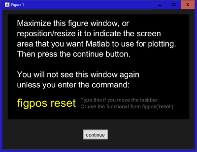
If called without an argument, screencfg attempts to determine the current screen borders automatically. For Windows based systems it does this by calling the auxiliary function workingArea.m (described below). For non-Windows based systems it does this using the WindowState property except for with older versions of Matlab which don't have this property. In that case it will use a java frame. In unusual situations (for example with a non-Windows sytems and a very old Matlab version such as Matlab 6), the automatic procedure may fail. In that case, a manual method is used where a figure appears and the user must manually maximize the figure using the maximize button in the figure title bar.
screenfig returns a 4 element vector specifying the region where plots can be positioned without covering up any portion of the taskbar. It also saves this 4 element vector in the screenfig appdata of the root object and also saves the vector in a file called screencfg.txt in the plt\ini folder. This ensures that the calculations required to determine the screen configuration only have to be done once.
If you want screencfg to recalculate the screen configuration (for example after the taskbar has been moved, type the command figpos reset (or the equivalent functional form figpos('reset')). This will delete the screen configuration information saved by this function as well as the information saved by the workingArea.m helper function, so that the screen configuration is recomputed the next time screencfg is called.
If you call screencfg with any argument, for example screencfg('manual') then the manual method is always used instead of any of the automatic methods. One advantage of the manual method is that instead of maximizing the figure that appears you can resize and reposition the figure to cover the region where you want plots to appear. In that way you can restrict the area to be used for plotting, which is not possible with the automatic methods (although the need for this is somewhat unusual). Note that even when called with an argument, screencfg will still use a previous calculation of the screen configuration unless you first call figpos('reset').
The figure shown here will appear when the manual screen configuration is being used. Simply maximize the figure and then press the continue button. Alternatively (as mentioned above) you can specify a region smaller than the maximized figure, by moving and resizing the figure before pressing the continue button.
workingArea(find usable screen area) |
| creates a figure filling the entire usable screen area. | |
| v = workingArea + [8 8 -16 -16]; figure('OuterPosition',v); |
similar to above, except it gives you an 8-pixel margin on all sides |
| w = workingArea; p = [380 250]; figure('OuterPosition',[w(1:2) p]); |
creates a 380 by 250 figure in the lower left corner of the working area |
| w = workingArea; p = [380 250]; v = [w(1)+w(3)-380 w(2) p]; figure('OuterPosition',v); |
creates a 380 by 250 figure in the lower right corner of the working area |
| w = workingArea; p = [380 250]; v = [w(1) w(2)+w(4)-250 p]; figure('OuterPosition',v); |
creates a 380 by 250 figure in the upper left corner of the working area |
| w = workingArea; p = [380 250]; v = [w(1:2)+w(3:4)-p p]; figure('OuterPosition',v); |
creates a 380 by 250 figure in the upper right corner of the working area |
| w = workingArea; v = [w(1)+w(3)-300 w(2) 300 w(4)]; figure('OuterPosition',v); |
creates the tallest 300-pixel wide figure as far to the right as possible |
| w = workingArea; v = [w(1) w(2)+w(4)-200 w(3) 200]; figure('OuterPosition',v); |
creates the widest 200-pixel high figure as far to the top as possible |
When called without an argument (as in the examples above) a 4-element row vector [x y width height] is returned.
When called with an argument, a scalar is returned. For example:
width = workingArea(3);
height = workingArea(4);
is equivalent to
w = workingArea; width = w(3); height = w(4);
These commands do not work with non-Windows operating systems or for Windows 8 or earlier, but figpos (described above) will give similar results and works with all operating systems. figpos returns values related to the inner position so they are somewhat smaller. For example figpos('width') is about 16 pixels smaller than workingArea(3) because it doesn't include the figure window border on the left and right. Also figpos('height') is about 40 pixels smaller than workingArea(4) because it doesn't include the figure window borders as well as the figure's title bar at the top of the figure.
As with figpos, workingArea will stop working correctly if you move or resize the taskbar. To fix that problem, type figpos('reset') in the command window. This will cause workingArea and figpos to recalculate the screen configuration based on the new taskbar position.
uic.m(createuicontrols) |
uic('Pos',{p1 p2 p3},'string','QRA');
will create 3 buttons, all with the same name (QRA) located at p1, p2, p3 where p1, p2, p3, are each a 4-element row vector specifying the button position [left bottom width height]. Of course, it is somewhat unusual to give the same name to each button, so here is another command to give the 3 buttons different names:
uic('Pos',{p1 p2 p3},'String',{'QRK' 'QRS' 'QSA'});
Notice that both properties are capitalized, meaning that both the Pos and String properties are distributed, so that each button has different positions and string values. Now suppose I want the 3 objects to be text uicontrols instead of buttons. Just add the style property to the command:
uic('Pos',{p1 p2 p3},'String',{'QRK' 'QRS' 'QSA'},'style','text');
Notice that style is lowercase, so that property value ('text') will be applied to all 3 objects. In fact, if you had capitalized 'style', uic would give you an error message since it would expect the argument to be a cell array.
Now if we change 'String' to 'string' in the above command we will get a quite different result. Since 'string' is now lower case it will assign the entire cell array to each text uicontrol which will create 3 controls all with the same multiline string containing the 3 lines QRK, QRS, and QSA.
h = uic( ... ); will return the handle of the control if a single control was created. If multiple controls were created, h will be a column vector containing the control handles.
[h1 h2 h3] = uic( ... ); will assign h1 to the first control, h2 to the 2nd, and h3 to the third ... assuming that the uic command produces exactly 3 objects. When supplying more than one argument, you will get an error message if the number of output arguments is not the same as the number of objects created.
See the following programs for examples of the use of the uic function:
| demo folder: | demoplt, gui1, movbar, pltmap, pltn, pub0, trigplt |
| math folder: | airspeed, carlo, curves, gauss, gpsLog, motion |
| sig folder: | afilt, editz, erip, winplt |
| util folder: | pltwater |